Vitalik: Binius, efficient proofs for binary fields

Original article by: Vitalik Buterin

Original translation: Kate, MarsBit

This post is primarily for readers who are generally familiar with 2019-era cryptography, and SNARKs and STARKs in particular. If you are not, I recommend reading those first. Special thanks to Justin Drake, Jim Posen, Benjamin Diamond, and Radi Cojbasic for their feedback and comments.

Over the past two years, STARKs have become a key and irreplaceable technology for efficiently making easily verifiable cryptographic proofs of very complex statements (e.g. proving that an Ethereum block is valid). One of the key reasons for this is the small field size: SNARKs based on elliptic curves require you to work on 256-bit integers to be secure enough, while STARKs allow you to use much smaller field sizes with greater efficiency: first the Goldilocks field (64-bit integer), then Mersenne 31 and BabyBear (both 31 bits). Due to these efficiency gains, Plonky 2 using Goldilocks is hundreds of times faster than its predecessors at proving many kinds of computations.

A natural question is: can we take this trend to its logical conclusion and build proof systems that run faster by operating directly on zeros and ones? This is exactly what Binius attempts to do, using a number of mathematical tricks that make it very different from SNARKs and STARKs from three years ago. This post describes why small fields make proof generation more efficient, why binary fields are uniquely powerful, and the tricks Binius uses to make proofs on binary fields so efficient.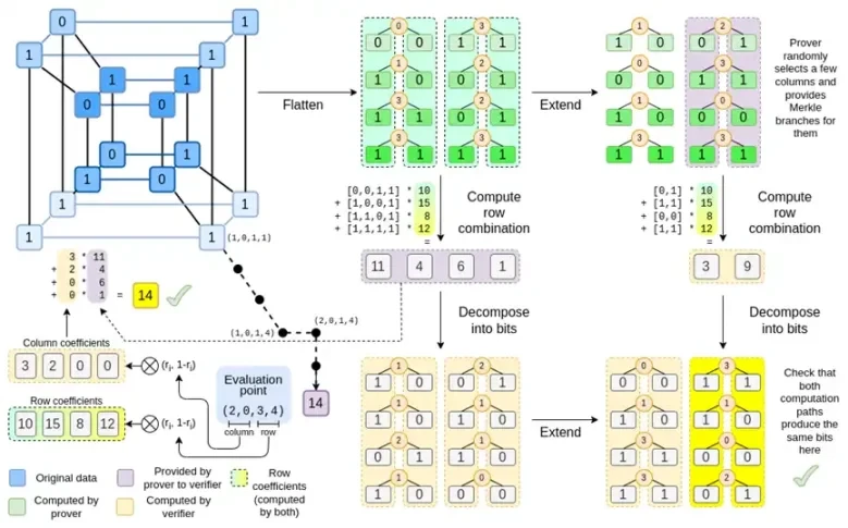

Binius, by the end of this post, you should be able to understand every part of this diagram.

Review: finite fields

One of the key tasks of cryptographic proof systems is to operate on large amounts of data while keeping the numbers small. If you can compress a statement about a large program into a mathematical equation containing a few numbers, but those numbers are as large as the original program, then you have gained nothing.

To do complex arithmetic while keeping numbers small, cryptographers often use modular arithmetic. We choose a prime number modulus p. The % operator means take the remainder: 15% 7 = 1, 53% 10 = 3, and so on. (Note that the answer is always non-negative, so for example -1% 10 = 9)

You may have seen modular arithmetic in the context of adding and subtracting time (e.g., what time is it 4 hours after 9?). But here, we don’t just add and subtract modulo a number; we can also multiply, divide, and take exponents.

We redefine: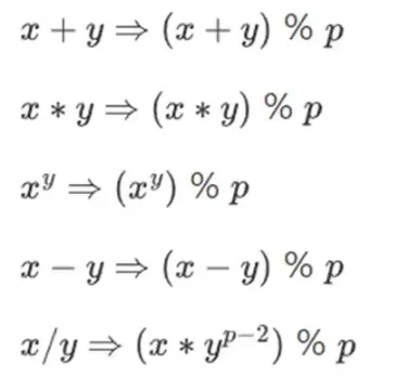

The above rules are all self-consistent. For example, if p = 7, then:

5 + 3 = 1 (because 8% 7 = 1)

1-3 = 5 (because -2% 7 = 5)

2* 5 = 3

3/5 = 2

A more general term for such structures is finite fields. A finite field is a mathematical structure that follows the usual laws of arithmetic, but in which the number of possible values is finite, so that each value can be represented by a fixed size.

Modular arithmetic (or prime fields) is the most common type of finite field, but there is another type: extension fields. You may have seen one extension field: the complex numbers. We imagine a new element and label it i, and do math with it: (3i+2)*(2i+4)=6i*i+12i+4i+8=16i+2. We can do the same with the extension of the prime field. As we start dealing with smaller fields, the extension of prime fields becomes increasingly important for security, and binary fields (used by Binius) rely entirely on extension to have practical utility.

Review: Arithmeticization

The way SNARKs and STARKs prove computer programs is through arithmetic: you take a statement about the program you want to prove, and turn it into a mathematical equation involving a polynomial. A valid solution to the equation corresponds to a valid execution of the program.

As a simple example, suppose I calculated the 100th Fibonacci number and I want to prove to you what it is. I create a polynomial F that encodes the Fibonacci sequence: so F(0)=F(1)=1, F(2)=2, F(3)=3, F(4)=5 and so on for 100 steps. The condition I need to prove is that F(x+2)=F(x)+F(x+1) over the entire range x={0, 1…98}. I can convince you by giving you the quotient:

where Z(x) = (x-0) * (x-1) * …(x-98). . If I can provide that F and H satisfy this equation, then F must satisfy F(x+ 2)-F(x+ 1)-F(x) in the range. If I additionally verify that for F, F(0)=F(1)=1, then F(100) must actually be the 100th Fibonacci number.

If you want to prove something more complicated, then you replace the simple relation F(x+2) = F(x) + F(x+1) with a more complicated equation that basically says F(x+1) is the output of initializing a virtual machine with state F(x), and run one computational step. You can also replace the number 100 with a larger number, for example, 100000000, to accommodate more steps.

All SNARKs and STARKs are based on the idea of using simple equations over polynomials (and sometimes vectors and matrices) to represent large numbers of relationships between individual values. Not all algorithms check for equivalence between adjacent computational steps like the above: for example, PLONK does not, and neither does R1CS. But many of the most effective checks do so, because it is easier to minimize overhead by performing the same check (or the same few checks) many times.

Plonky 2: From 256-bit SNARKs and STARKs to 64-bit… only STARKs

Five years ago, a reasonable summary of the different types of zero-knowledge proofs was as follows. There are two types of proofs: (elliptic curve-based) SNARKs and (hash-based) STARKs. Technically, STARKs are a type of SNARK, but in practice, it’s common to use “SNARK” to refer to the elliptic curve-based variant and “STARK” to refer to the hash-based construction. SNARKs are small, so you can verify them very quickly and install them on-chain easily. STARKs are large, but they don’t require a trusted setup, and they’re quantum-resistant.

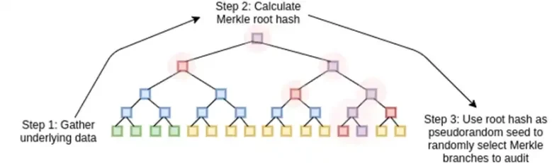
STARKs work by treating data as a polynomial, computing the computation of that polynomial, and using the Merkle root of the extended data as a “polynomial commitment”.

A key piece of history here is that elliptic curve-based SNARKs were widely used first: STARKs didn’t become efficient enough until around 2018, thanks to FRI, and by then Zcash had been running for over a year. Elliptic curve-based SNARKs have a key limitation: if you want to use an elliptic curve-based SNARK, then the arithmetic in these equations must be done modulo the number of points on the elliptic curve. This is a large number, usually close to 2 to the power of 256: for example, for the bn128 curve it’s 21888242871839275222246405745257275088548364400416034343698204186575808495617. But real computing uses small numbers: if you think about a real program in your favorite language, most of the things it uses are counters, indexes in for loops, positions in the program, single bits representing True or False, and other things that are almost always only a few digits long.

Even if your original data consists of small numbers, the proof process requires computing quotients, expansions, random linear combinations, and other data transformations that will result in an equal or larger number of objects that are on average as large as the full size of your field. This creates a key inefficiency: to prove a computation on n small values, you have to do many more computations on n much larger values. Initially, STARKs inherited the SNARK habit of using 256-bit fields, and thus suffered from the same inefficiency.

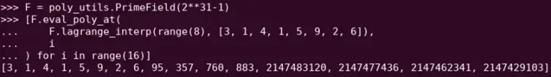
Reed-Solomon expansion of some polynomial evaluation. Even though the original value is small, the additional values are expanded to the full size of the field (in this case 2^31 – 1)

In 2022, Plonky 2 was released. The main innovation of Plonky 2 is to do arithmetic modulo a smaller prime number: 2 to the power of 64 – 2 to the power of 32 + 1 = 18446744067414584321. Now, each addition or multiplication can always be done in a few instructions on the CPU, and hashing all the data together is 4 times faster than before. But there is a problem: this method only works for STARKs. If you try to use SNARKs, elliptic curves become insecure for such small elliptic curves.

To ensure security, Plonky 2 also needs to introduce extension fields. A key technique for checking arithmetic equations is random point sampling: if you want to check whether H(x) * Z(x) is equal to F(x+ 2)-F(x+ 1)-F(x), you can randomly choose a coordinate r, provide a polynomial commitment to prove H(r), Z(r), F(r), F(r+ 1) and F(r+ 2), and then verify whether H(r) * Z(r) is equal to F(r+ 2)-F(r+ 1)- F(r). If an attacker can guess the coordinates in advance, then the attacker can deceive the proof system – this is why the proof system must be random. But this also means that the coordinates must be sampled from a large enough set that the attacker cannot guess randomly. This is obviously true if the modulus is close to 2 to the power of 256. However, for the modulus 2^64 – 2^32 + 1, we are not there yet, and this is certainly not the case if we get down to 2^31 – 1. It is well within the capabilities of an attacker to try to forge a proof two billion times until one gets lucky.

To prevent this, we sample r from an extended field, so that, for example, you can define y where y^3 = 5, and take combinations of 1, y, and y^2. This brings the total number of coordinates to about 2^93. Most of the polynomials computed by the prover dont go into this extended field; theyre just integers modulo 2^31-1, so you still get all the efficiency from using a small field. But random point checks and FRI computations do reach into this larger field to get the security they need.

From small prime numbers to binary numbers

Computers do arithmetic by representing larger numbers as sequences of 0s and 1s, and building circuits on top of those bits to compute operations like addition and multiplication. Computers are particularly optimized for 16-, 32-, and 64-bit integers. For example, 2^64 – 2^32 + 1 and 2^31 – 1 were chosen not only because they fit within those bounds, but also because they fit well within those bounds: multiplication modulo 2^64 – 2^32 + 1 can be performed by doing a regular 32-bit multiplication, and bitwise shifting and copying the output in a few places; this article explains some of the tricks nicely.

However, a much better approach would be to do the calculations directly in binary. What if addition could be just XOR, without having to worry about carryover from adding 1 + 1 from one bit to the next? What if multiplication could be more parallelized in the same way? These advantages are all based on being able to represent true/false values with a single bit.

Getting these advantages of doing binary computation directly is exactly what Binius is trying to do. The Binius team demonstrated the efficiency gains in their presentation at zkSummit:

Despite being roughly the same size, operations on 32-bit binary fields require 5 times less computational resources than operations on 31-bit Mersenne fields.

From univariate polynomials to hypercubes

Suppose we believe this reasoning, and want to do everything with bits (0 and 1). How can we represent a billion bits with a single polynomial?

Here we face two practical problems:

1. For a polynomial to represent a large number of values, these values need to be accessible when evaluating the polynomial: in the Fibonacci example above, F(0), F(1) … F(100), and in a larger calculation, the exponents will be in the millions. The fields we use need to contain numbers of this size.

2. Proving any value we commit in a Merkle tree (like all STARKs) requires Reed-Solomon encoding it: for example, expanding the values from n to 8n, using redundancy to prevent malicious provers from cheating by forging a value during the calculation. This also requires having a large enough field: to expand from a million values to 8 million, you need 8 million different points to evaluate the polynomial.

A key idea of Binius is to solve these two problems separately, and do so by representing the same data in two different ways. First, the polynomials themselves. Systems like elliptic curve-based SNARKs, 2019-era STARKs, Plonky 2, and others typically deal with polynomials over one variable: F(x). Binius, on the other hand, takes inspiration from the Spartan protocol and uses multivariate polynomials: F(x 1, x 2,… xk). In effect, we represent the entire computational trajectory on a hypercube of computation, where each xi is either 0 or 1. For example, if we want to represent a Fibonacci sequence, and we still use a field large enough to represent them, we can imagine their first 16 sequences like this: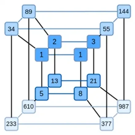

That is, F(0,0,0,0) should be 1, F(1,0,0,0) is also 1, F(0,1,0,0) is 2, and so on, all the way up to F(1,1,1,1) = 987. Given such a hypercube of computations, there is a multivariate linear (degree 1 in each variable) polynomial that produces these computations. So we can think of this set of values as representing the polynomial; we dont need to compute the coefficients.

This example is of course just for illustration: in practice, the whole point of going into the hypercube is to let us deal with individual bits. The Binius-native way to compute Fibonacci numbers is to use a higher-dimensional cube, storing one number per group of, say, 16 bits. This requires some cleverness to implement integer addition on a bit basis, but for Binius, its not too hard.

Now, lets look at erasure codes. The way STARKs work is that you take n values, Reed-Solomon expand them to more values (usually 8n, usually between 2n and 32n), then randomly select some Merkle branches from the expansion and perform some kind of check on them. The hypercube has length 2 in each dimension. Therefore, it is not practical to expand it directly: there is not enough room to sample Merkle branches from 16 values. So how do we do it? Lets assume the hypercube is a square!

Simple Binius – An Example

See here for a python implementation of the protocol.

Lets look at an example, using regular integers as our fields for convenience (in a real implementation, wed use binary field elements). First, we encode the hypercube we want to submit as a square:

Now, we expand the square using the Reed-Solomon method. That is, we treat each row as a degree 3 polynomial evaluated at x = { 0, 1, 2, 3 } and evaluate the same polynomial at x = { 4, 5, 6, 7 }: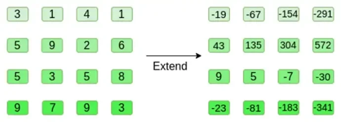

Note that the numbers can get really big! This is why in practical implementations we always use finite fields, rather than regular integers: if we use integers modulo 11, for example, the expansion of the first row will just be [3, 10, 0, 6].

If you want to try out the extension and verify the numbers yourself, you can use my simple Reed-Solomon extension code here.

Next, we treat this extension as a column and create a Merkle tree of the column. The root of the Merkle tree is our commitment.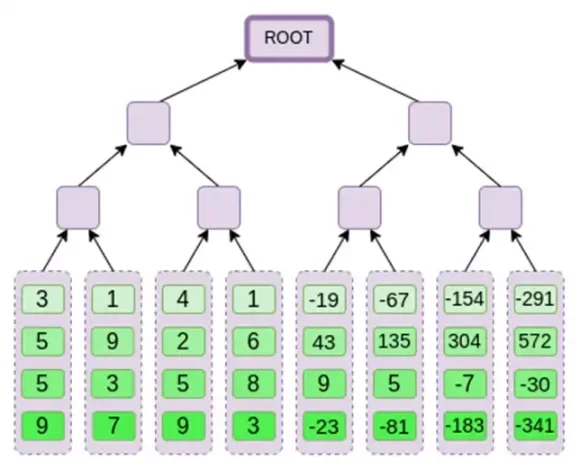

Now, lets assume that the prover wants to prove the computation of this polynomial r = {r 0, r 1, r 2, r 3 } at some point. There is a subtle difference in Binius that makes it weaker than other polynomial commitment schemes: the prover should not know or be able to guess s before committing to the Merkle root (in other words, r should be a pseudo-random value that depends on the Merkle root). This makes the scheme useless for database lookups (e.g., ok, you gave me the Merkle root, now prove to me P(0, 0, 1, 0)!). But the zero-knowledge proof protocols we actually use usually dont require database lookups; they only require checking the polynomial at a random evaluation point. So this restriction serves our purposes well.

Suppose we choose r = { 1, 2, 3, 4 } (the polynomial evaluates to -137; you can confirm this using this code). Now, we get to the proof. We split r into two parts: the first part { 1, 2 } represents the linear combination of the columns within the row, and the second part { 3, 4 } represents the linear combination of the rows. We compute a tensor product and for the columns:

For the row part:

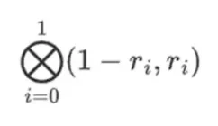
This means: a list of all possible products of a value in each set. In the row case, we get:

[( 1-r 2)*( 1-r 3), ( 1-r 3), ( 1-r 2)*r 3, r 2*r 3 ]

With r = { 1, 2, 3, 4 } (so r 2 = 3 and r 3 = 4):

[( 1-3)*( 1-4), 3*( 1-4),( 1-3)* 4, 3* 4 ] = [ 6, -9 -8 -12 ]

Now, we compute a new row t by taking a linear combination of the existing rows. That is, we take:

You can think of whats happening here as a partial evaluation. If we multiplied the full tensor product by the full vector of all values, youd get the computation P(1, 2, 3, 4) = -137. Here, weve multiplied the partial tensor product using only half of the evaluation coordinates, and reduced the grid of N values to a single row of square root N values. If you give this row to someone else, they can do the rest of the computation using the tensor product of the other half of the evaluation coordinates.

The prover provides the verifier with the following new row: t and a Merkle proof of some randomly sampled columns. In our illustrative example, we will have the prover provide only the last column; in real life, the prover would need to provide dozens of columns to achieve adequate security.

Now, we exploit the linearity of Reed-Solomon codes. The key property we exploit is that taking a linear combination of Reed-Solomon expansions gives the same result as taking a Reed-Solomon expansion of a linear combination. This sequential independence usually occurs when both operations are linear.

The verifier does exactly that. They compute t, and compute linear combinations of the same columns that the prover computed before (but only the columns provided by the prover), and verify that the two procedures give the same answer.

In this case, we expand t and compute the same linear combination ([6,-9,-8, 12]), which both give the same answer: -10746. This proves that the Merkle root was constructed in good faith (or at least close enough), and that it matches t: at least the vast majority of the columns are compatible with each other.

But there is one more thing the verifier needs to check: check the evaluation of the polynomial {r 0 …r 3 }. All the steps of the verifier so far have not actually depended on the value claimed by the prover. Here is how we check it. We take the tensor product of the “column part” that we marked as the computation point:

In our case, where r = { 1, 2, 3, 4 } so the half of the columns selected is { 1, 2 }), this is equivalent to:

Now we take this linear combination t:

This is the same as directly solving the polynomial.

The above is very close to a complete description of the simple Binius protocol. This already has some interesting advantages: for example, since the data is separated into rows and columns, you only need a field that is half the size. However, this does not achieve the full benefits of computing in binary. For that, we need the full Binius protocol. But first, lets take a deeper look at binary fields.

Binary Fields

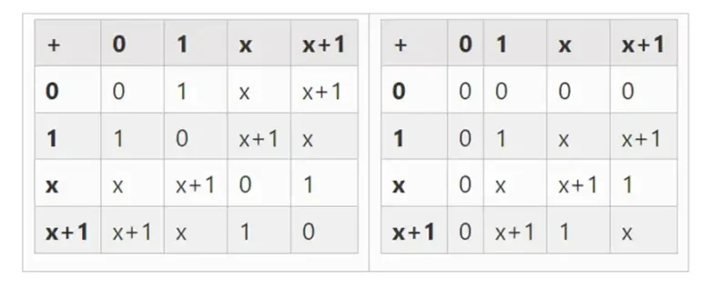
The smallest possible field is arithmetic modulo 2, which is so small that we can write addition and multiplication tables for it:

We can get larger binary fields by extension: if we start with F 2 (integers modulo 2) and then define x where x squared = x + 1 , we get the following addition and multiplication tables:

It turns out that we can extend binary fields to arbitrarily large sizes by repeating this construction. Unlike complex numbers over the real numbers, where you can add a new element but never add any more elements I (quaternions do exist, but they are mathematically weird, e.g. ab is not equal to ba), with finite fields you can add new extensions forever. Specifically, our definition of an element is as follows: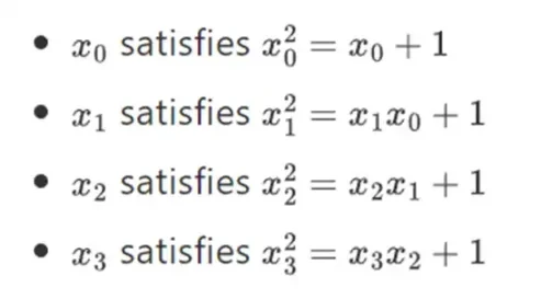

And so on… This is often called a tower construction, because each successive expansion can be thought of as adding a new layer to the tower. This is not the only way to construct binary fields of arbitrary size, but it has some unique advantages that Binius exploits.

We can represent these numbers as lists of bits. For example, 1100101010001111. The first bit represents multiples of 1, the second bit represents multiples of x0, and then the following bits represent multiples of x1: x1, x1*x0, x2, x2*x0, and so on. This encoding is nice because you can break it down:

This is a relatively uncommon notation, but I like to represent binary field elements as integers, with the more efficient bit on the right. That is, 1 = 1, x0 = 01 = 2, 1+x0 = 11 = 3, 1+x0+x2 = 11001000 = 19, and so on. In this representation, thats 61779.

Addition in the binary field is just XOR (and so is subtraction, by the way); note that this means x+x = 0 for any x. To multiply two elements x*y together, there is a very simple recursive algorithm: split each number in half:

Then, split the multiplication:

The last part is the only one thats a little tricky, because you have to apply simplification rules. There are more efficient ways to do the multiplication, similar to Karatsubas algorithm and Fast Fourier Transforms, but Ill leave that as an exercise for the interested reader to figure out.

Division in binary fields is done by combining multiplication and inversion. The simple but slow inversion method is an application of the generalized Fermats little theorem. There is also a more complex but more efficient inversion algorithm that you can find here. You can use the code here to play with addition, multiplication, and division of binary fields.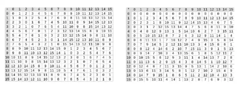

Left: Addition table for four-bit binary field elements (i.e., only 1, x 0, x 1, x 0x 1). Right: Multiplication table for four-bit binary field elements.

The beauty of this type of binary field is that it combines some of the best parts of regular integers and modular arithmetic. Like regular integers, binary field elements are unbounded: you can grow as large as you want. But just like modular arithmetic, if you operate on values within a certain size limit, all your results will stay in the same range. For example, if you take 42 to successive powers, you get:

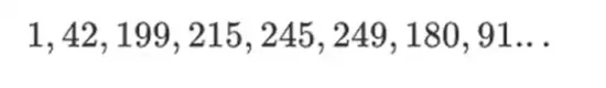
After 255 steps, you are back to 42 to the power of 255 = 1, and just like positive integers and modular operations, they obey the usual laws of mathematics: a*b=b*a, a*(b+c)=a*b+a*c, and even some weird new laws.

Finally, binary fields are convenient for manipulating bits: if you do math with numbers that fit in 2k, then all your output will fit in 2k bits as well. This avoids awkwardness. In Ethereums EIP-4844, the individual blocks of a blob must be numbers modulo 52435875175126190479447740508185965837690552500527637822603658699938581184513, so encoding binary data requires throwing away some space and doing extra checks at the application layer to ensure that the value stored in each element is less than 2248. This also means that binary field operations are super fast on computers – both CPUs and theoretically optimal FPGA and ASIC designs.

This all means that we can do Reed-Solomon encoding like we did above, in a way that completely avoids integer explosion as we saw in our example, and in a very native way, the kind of computations that computers are good at. The split property of binary fields – how we can do 1100101010001111 = 11001010 + 10001111*x 3 , and then split it up as we need – is also crucial to allow for a lot of flexibility.

Complete Binius

See here for a python implementation of the protocol.

Now we can move on to “full Binius,” which adapts “simple Binius” to (i) work on binary fields and (ii) let us commit single bits. This protocol is hard to understand because it switches back and forth between different ways of looking at matrices of bits; it certainly took me longer to understand it than it usually takes me to understand cryptographic protocols. But once you understand binary fields, the good news is that the “harder math” that Binius relies on doesn’t exist. This isn’t elliptic curve pairings, where there are deeper and deeper algebraic geometry rabbit holes to go down; here, you just have binary fields.

Lets look at the full chart again:

By now, you should be familiar with most of the components. The idea of flattening a hypercube into a grid, the idea of computing row and column combinations as tensor products of evaluation points, and the idea of checking the equivalence between Reed-Solomon expansion then computing row combinations and computing row combinations then Reed-Solomon expansion are all implemented in plain Binius.

Whats new in Complete Binius? Basically three things:

• The individual values in the hypercube and square must be bits (0 or 1).

• The expansion process expands the bits into more bits by grouping them into columns and temporarily assuming that they are elements of a larger field.

• After the row combination step, there is an element-wise decomposition to bits step that converts the expansion back to bits.

Well discuss both cases in turn. First, the new extension procedure. Reed-Solomon codes have a fundamental limitation, if you want to extend n to k*n, you need to work in a field with k*n different values that can be used as coordinates. With F 2 (aka bits), you cant do that. So what we do is, pack adjacent elements of F 2 together to form larger values. In the example here, we pack two bits at a time into the elements { 0 , 1 , 2 , 3 } , which is enough for us since our extension only has four computation points. In a real proof, we might go back 16 bits at a time. We then execute the Reed-Solomon code on these packed values and unpack them into bits again.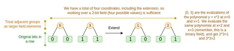

Now, row combinations. In order to make the evaluate at a random point check cryptographically secure, we need to sample that point from a fairly large space (much larger than the hypercube itself). So while the point inside the hypercube is the bit, the computed value outside the hypercube will be much larger. In the example above, the row combination ends up being [11, 4, 6, 1].

This presents a problem: we know how to group bits into a larger value and then perform a Reed-Solomon expansion on that value, but how do we do the same thing for larger pairs of values?

Binius trick is to do it bit by bit: we look at a single bit of each value (e.g., for the thing we labeled 11, thats [1, 1, 0, 1]), and then we expand it row by row. That is, we expand it on the 1 row of each element, then on the x0 row, then on the x1 row, then on the x0x1 row, and so on (well, in our toy example we stop there, but in a real implementation wed go up to 128 rows (the last one being x6*…*x0))

review:

• We convert the bits in the hypercube into a grid

• We then treat groups of adjacent bits on each row as elements of a larger field and perform arithmetic operations on them to Reed-Solomon expand the row

• We then take the row combination of each column of bits and get the column of bits for each row as output (much smaller for squares larger than 4 x 4)

• Then, we consider the output as a matrix and its bits as rows

Why is this happening? In normal math, if you start slicing a number bit by bit, the (usual) ability to do linear operations in any order and get the same result breaks down. For example, if I start with the number 345, and I multiply it by 8, then by 3, I get 8280, and if I do those two operations in reverse, I also get 8280. But if I insert a bit-slicing operation between the two steps, it breaks down: if you do 8x, then 3x, you get: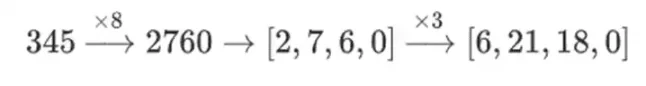

But if you do 3x, then 8x, you get:

But in binary fields built with tower structures, this approach does work. The reason is their separability: if you multiply a large value by a small value, what happens on each segment stays on each segment. If we multiply 1100101010001111 by 11, this is the same as the first decomposition of 1100101010001111, which is

Then multiply each component by 11.

Putting it all together

In general, zero-knowledge proof systems work by making statements about a polynomial that represent statements about the underlying evaluation at the same time: just like we saw in the Fibonacci example, F(X+ 2)-F(X+ 1)-F(X) = Z(X)*H(X) while checking all steps of the Fibonacci calculation. We check statements about the polynomial by proving the evaluation at random points. This check of random points represents a check of the entire polynomial: if the polynomial equation doesnt match, there is a small chance that it matches at a specific random coordinate.

In practice, one major source of inefficiency is that in real programs, most of the numbers we deal with are small: indices in for loops, True/False values, counters, and things like that. However, when we extend data with Reed-Solomon encoding to provide the redundancy required to make Merkle-proof-based checks secure, most of the extra values end up taking up the entire size of the field, even if the original value was small.

To fix this, we want to make this field as small as possible. Plonky 2 took us from 256-bit numbers to 64-bit numbers, and then Plonky 3 dropped it further to 31 bits. But even that is not optimal. With binary fields, we can deal with single bits. This makes the encoding dense: if your actual underlying data has n bits, then your encoding will have n bits, and the expansion will have 8*n bits, with no additional overhead.

Now, lets look at this chart a third time:

In Binius, we work on a multilinear polynomial: a hypercube P(x0, x1,…xk) where the single evaluations P(0, 0, 0, 0), P(0, 0, 0, 1) up to P(1, 1, 1, 1), hold the data we care about. To prove a computation at a certain point, we reinterpret the same data as a square. We then extend each row, using Reed-Solomon encoding to provide the data redundancy required for security against randomized Merkle branch queries. We then compute random linear combinations of the rows, designing the coefficients so that the new combined row actually contains the computed value we care about. This newly created row (reinterpreted as a 128-bit row) and some randomly selected columns with Merkle branches are passed to the verifier.

The verifier then performs the extended row combination (or more precisely, the extended columns) and the extended row combination and verifies that the two match. It then computes a column combination and checks that it returns the value claimed by the prover. This is our proof system (or more precisely, the polynomial commitment scheme, which is a key component of the proof system).

What haven’t we covered yet?

• An efficient algorithm to expand the rows is required to actually make the validator computationally efficient. We use the Fast Fourier Transform on binary fields, described here (although the exact implementation will be different, as this post uses a less efficient construction that is not based on recursive expansion).

• Arithmetically. Univariate polynomials are convenient because you can do things like F(X+2)-F(X+1)-F(X) = Z(X)*H(X) to link adjacent steps in the computation. In the hypercube, next step is much less well explained than X+1. You can do X+k, powers of k, but this jumping behavior sacrifices many of Binius key advantages. The Binius paper describes the solution. See Section 4.3), but this is a deep rabbit hole in itself.

• How to safely do specific value checks. The Fibonacci example required checking key boundary conditions: the values of F(0)=F(1)=1 and F(100). But for original Binius, it is unsafe to do checks at known calculation points. There are some fairly simple ways to convert known calculation checks to unknown calculation checks, using so-called sum-checking protocols; but we wont cover those here.

• Lookup protocols, another technology that has been widely used recently, are used to make super efficient proof systems. Binius can be used in conjunction with lookup protocols for many applications.

• Beyond square root verification time. Square roots are expensive: a Binius proof of 2^32 bits is about 11 MB long. You can compensate for this by using other proof systems to make proofs of Binius proofs, giving you the efficiency of a Binius proof with a smaller proof size. Another option is the more complex FRI-Binius protocol, which creates a proof of multi-logarithmic size (just like regular FRI).

• How Binius affects SNARK-friendliness. The basic summary is that if you use Binius, you no longer need to care about making computations arithmetic-friendly: regular hashing is no longer more efficient than traditional arithmetic hashing, multiplication modulo 2 to the power of 32 or modulo 2 to the power of 256 is no longer as painful as multiplication modulo 2, etc. But this is a complex topic. A lot of things change when everything is done in binary.

I expect to see more improvements in binary field based proof technology in the coming months.

This article is sourced from the internet: Vitalik: Binius, efficient proofs for binary fields

Related: BNB Coin Shows Recovery Signs: New Yearly High on Sight

In Brief BNB price bounced back from $550 to inch closer to breaching $593 resistance. The price indicators have regained the bullish momentum, which supports an 8% rise. Sharpe Ratio at 4.03 will likely drive new investors towards the exchange token. March was a favorable month for BNB Coin, with the cryptocurrency achieving two new highs for the year within just a few days before experiencing a correction. After a nearly two-week period of recovery, BNB Coin is showing signs of potentially reaching a new high in 2024. But is such a milestone achievable? BNB Looks Promising Following a rebound from the $550 support level, the value of BNB Coin has risen to $581 at the time of this analysis. This improvement reflects a recovery in the altcoin’s risk-return profile,…